Introduction to Neural Nets
If you’re reading this article you probably already know the benefits of neural nets (NN) and deep learning but maybe you want to obtain an understanding of how they work. You’ve come to the right place!
What surprised me most when learning about NNs for the first time was their mathematical simplicity. Despite NNs being on the frontier of breakthroughs in fields such as computer vision [1] and natural language processing [2,3], the inner workings of them are quite simple to understand.
In this article we will go through a description of how NN work by using the “Hello World!” equivalent of deep learning — handwritten digit recognition.
So let’s get straight into it.
NN —How do they work?
NNs contain two phases;
- Forward Propagation
- Back Propagation
During the training of a NN you perform both of these phases. When you would like the NN to make a prediction for an unlabelled example, you would simply perform forward propagation. Back propagation is really the magic that allows NN to perform so well for tasks that are traditionally very difficult for computers to carry out.
Forward Propagation
To give the NN some context we will consider one of the original problems it was applied to – handwritten digit recognition [4]. This problem is often one of the first encountered by students of Deep Learning as it represents a problem that is hard to solve with traditional machine learning methods.
Imagine that we are tasked to write a computer program that can identify handwritten digits. Each image we receive will be 28 x 28 pixels and we will also have access to the correct label for that image. The first thing we do is set up our neural network as in the figure below.
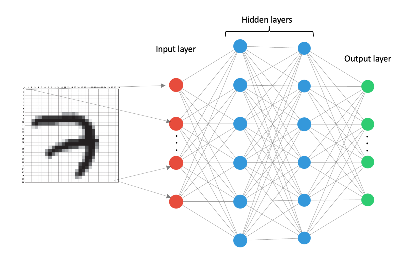

Each circle in Fig. 1 represents a ‘neuron’. A neuron simply holds a scalar value, i.e. a number. The red neurons define the input layer. This is where we will input our image. The blue neurons represent the hidden layers. They are called hidden layers because the user never interacts directly with these neurons. The green neurons represent the output layer. This is where the NN will output its prediction for what digit is in the image.
We have 784 pixels in total (28 x 28), so our input layer consists of 784 neurons. Let’s call the top red neuron in Fig. 1 neuron 1 and the bottom one neuron 784. The value of each neuron takes on the value of the pixel it is connected to. For example, if our image has a pixel depth of 8 bit, then a single pixel can take on a value between 0 and 256 (2⁸). 0 would represent a completely white pixel and 256 would represent a completely black pixel, with a sliding scale in between these values. The value of a neuron is called it’s activation. We will represent the activation of a neuron by the symbol a.
The next thing we do is we attach every neuron in the input layer to every neuron in the next layer. This is shown as grey lines in Fig. 1. We also add a weight to each of these connections. A weight, like the neuron’s value, is just a scalar value. Fig. 2 shows three of the weights labelled for our NN. Here the subscripts just help us to keep track of which two neurons the weight corresponds to. So for instance, the weight w31 is the weight for the connection between neuron 1 in the input layer and neuron 3 in the first hidden layer. The larger the weight between neurons the stronger the connection between them.
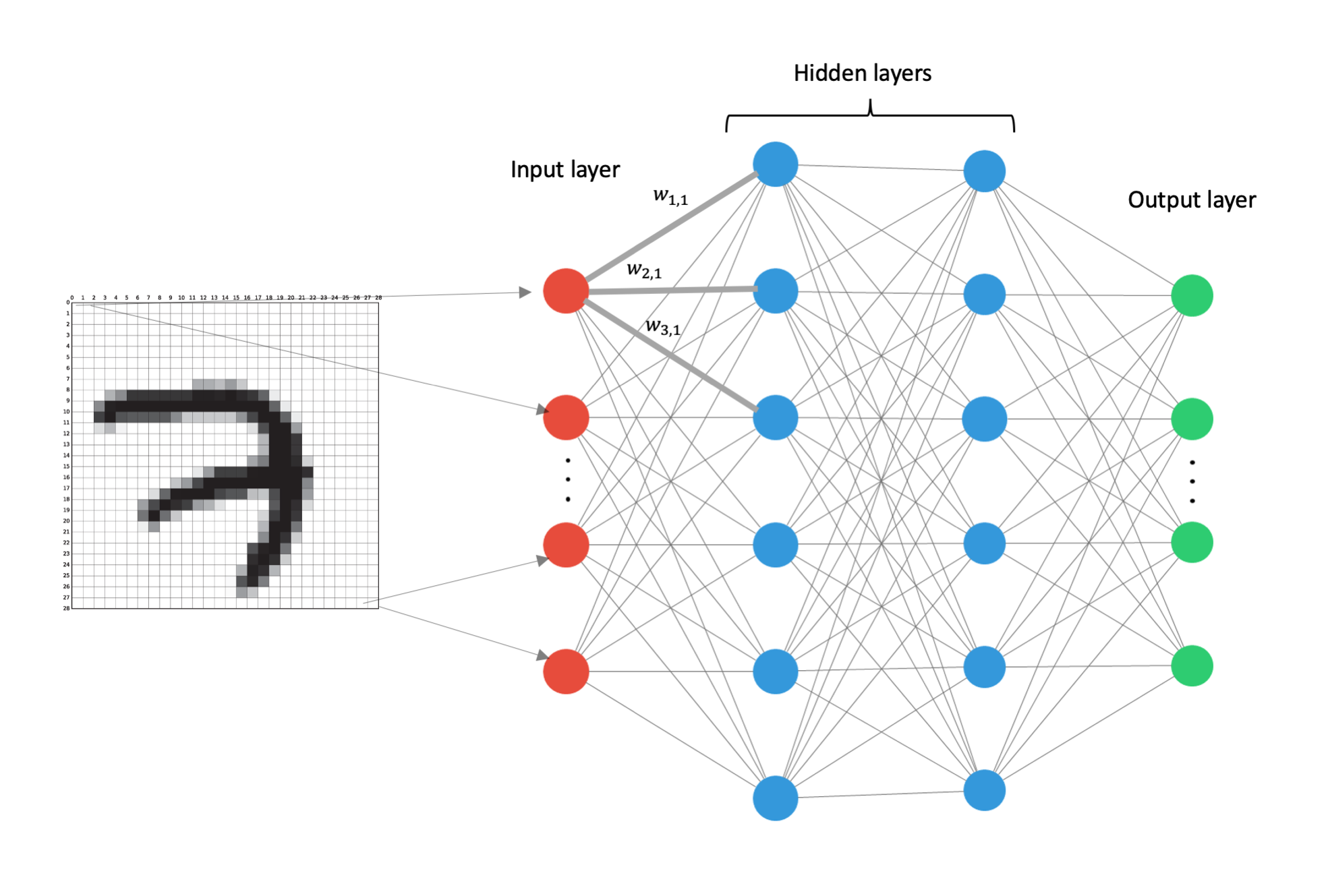

Now we need to work out the activation values of the neurons in the first hidden layer. We do this in two parts. In the first part we simply multiply the activation of each neuron in the previous layer by the weight that is attached to it. We then add all these terms up and add a ‘bias’ term which we denote b. Finally, we put this weighted sum through a nonlinear function such as tanh(x) or the sigmoid function which I will represent by σ. [See the “Questions” section if you’re interested in why we use a bias term and a nonlinear function.]
Let’s break this down a bit. If we consider what is happening at the first neuron in the hidden layer then we have what is displayed in Fig. 3.


This neuron has contributions from all the neurons in the first layer. Each of the neurons in the first layer come with their own weight which they are multiplied by. Then we add all these terms and add the single bias term. This weighted sum is represented by the symbol z₁² where the 1 shows that we are talking about the first neuron in the layer, and the 2 in the superscript denotes we are referring to the second layer in the network. Then this weighted sum is put through the nonlinear function to obtain the activation of the first neuron in the first hidden layer (second layer of the network), which we will call a₁².


We repeat this process for all neurons in the first hidden layer: multiplying each of the neurons from the input later by the weight connecting it to the neuron in the first hidden layer, adding a bias term, and then putting this weighted sum z into a nonlinear function.
Now that we have the activations for all the neurons in the first hidden layer, we repeat this process to get the activations for the neurons in the second hidden layer and then again to get the activations for the output layer. It is important to know that the weights between different layers are different.
Since our task is to predict the digit in the image, the output layer will contain 10 neurons representing the numbers 0,1,2,…,9. Each of the neurons in the final layer will contain a activation value between 0 and 1 and we take the neuron with the highest activation as the NNs guess as to what digit is in the image.
Before the NN has been trained, the network will most likely not be able to correctly identify what digit is in the image. For instance, consider the situation shown in Fig. 5.
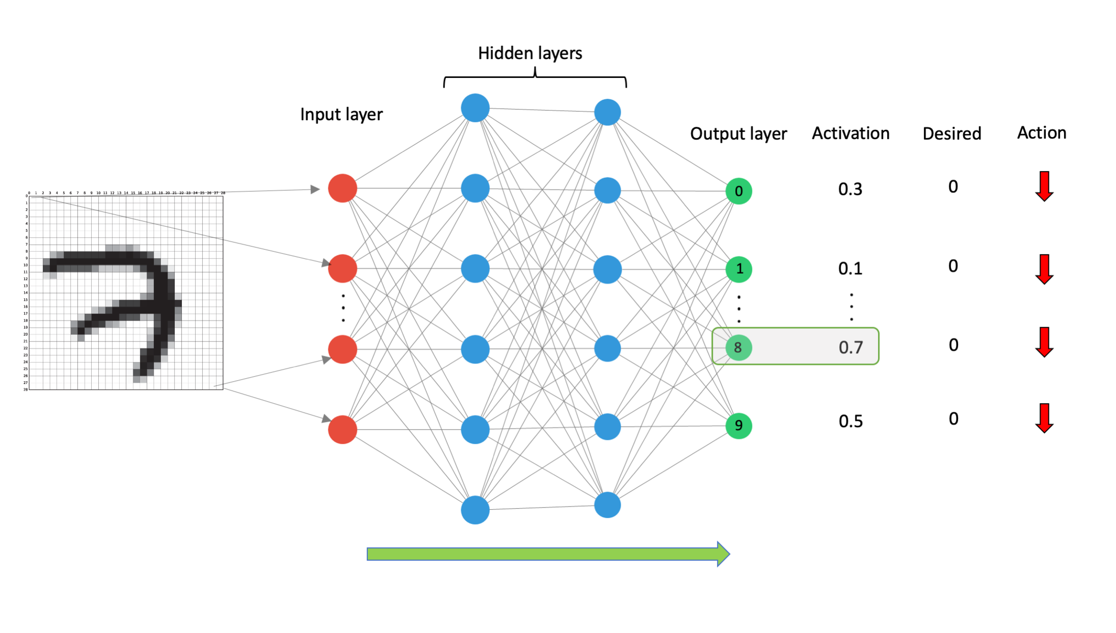

An image of the digit 7 was input into the NN and all of the activations calculated. What we see at the output layer is that the activation value for the neuron representing the digit 8 is highest and so the NN thinks that the digit 8 was in the image which clearly is wrong. So what we need to do is change the values of all the weights and all the biases so that the activations of all the neurons in the output layer are pushed towards 0 except for the neuron representing the digit 7.
With networks nowadays easily able to contain millions, and even billions, of weights and biases, how on Earth do we make all these changes to get us closer to the correct answer?
It turns out that we know, and have done for quite some time [5], a technique which very efficiently calculates the changes needed. This algorithm is called back propagation.
Back Propagation
To start adjusting our weights and biases to get the NN closer to the correct answer the first thing we need to do is define a cost function. A cost function just quantifies how wrong a system is. Let’s use mean squared error (MSE). To calculate the MSE for a single training example, we run our digit through our NN and calculate the difference between the activation of the neurons in the output layer and the desired activation. We then square these values, add them all up, and divide by the number of terms we added up which is 10 for our case.
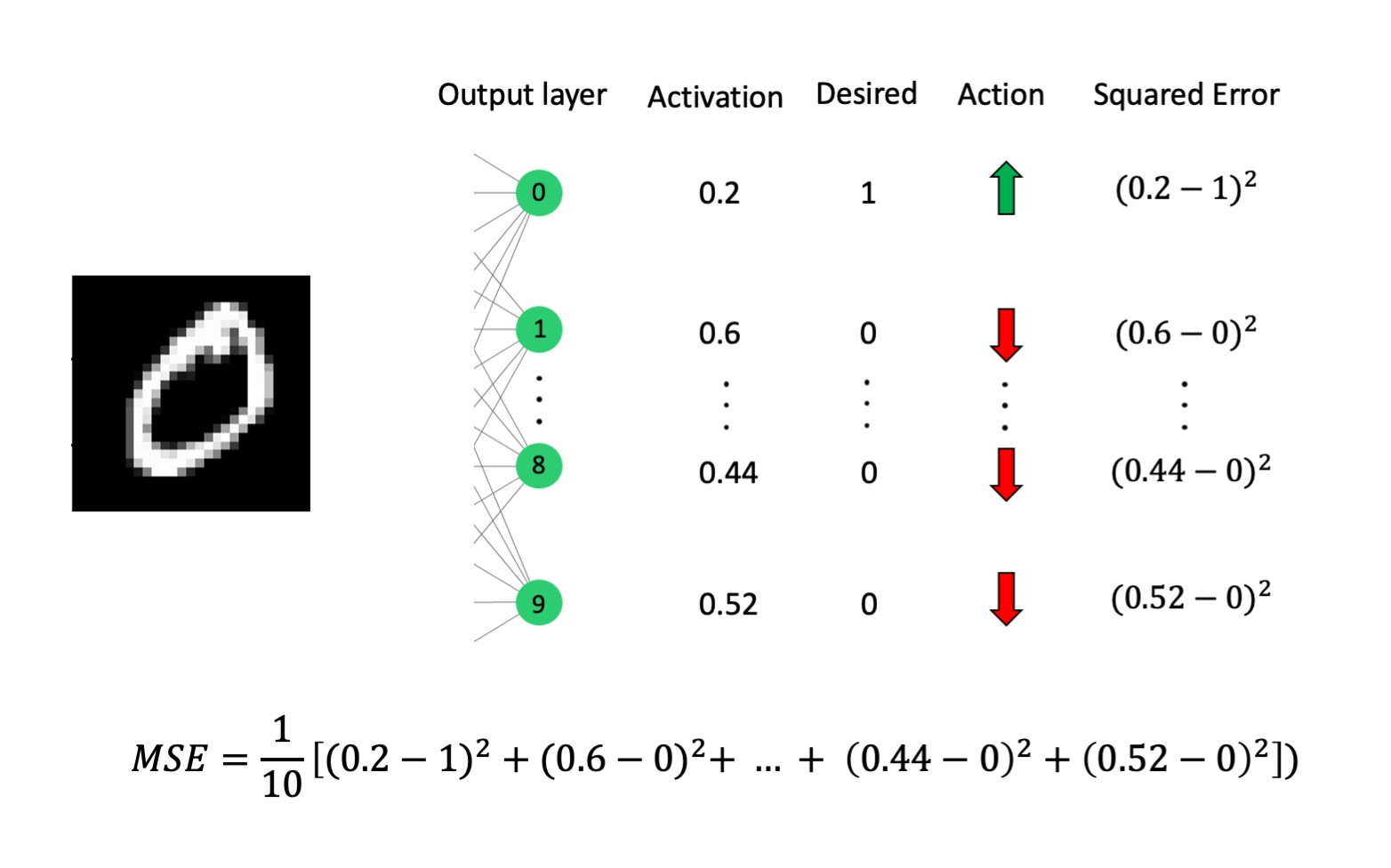

Fig. 6 shows the calculation of the cost function for a training example of the digit 0. This is the cost of a single training example. Then we run the rest of our training examples through the network and calculate all of their cost’s. We define a single number, called the average cost, to be the average of all the single example cost’s. For example, if we had 400 training examples, our average cost would be the sum of all the costs of the 400 examples, divided by 400. This gives us the average cost for 1 round of training (usually called an epoch), let’s represent this by C(w).
Now we want to change all of the weights and biases, so that this cost is as small as possible.
To better understand this, imagine the whole system is characterised by a single weight, instead of the thousands that we have at the moment. Then our cost function might look something like Fig. 7.


Plotted in red is the average cost, C(w), for different values of w. As stated before, we want to minimise C(w). In other words, we want to change w so that we get to the minimum of the red curve.
Also shown in Fig. 7 are two possible values for w as blues circles with their associated gradients as black dashed lines. What we can deduce from Fig. 7 is that we should move w to the right if the gradient at our current point is negative, and to the left if the gradient is positive.
Furthermore, we should move by an amount that is proportional to the gradient. If the gradient is large, we should move by a larger amount than if the gradient is small as this indicates that we are close to the minimum of the red curve. This logic can be summed up by the weight update equation.


NOTE: Remember that we do not know the exact surface of C(w) as shown in Fig. 7 otherwise we could simply change our weight to the optimal value to minimise C(w). We instead have to use our local measurement of the gradient to tells us which direction to move in to get us closer to the minimum.
The weight update equation tells us that the weights in the next training run (the next epoch) w(t+1) should be equal to the weights of the current run w(t) adjusted by the gradient dC(w)/dw of the current run. η is called the ‘learning rate’, and it controls how much influence the current gradient has on the weight update. It is usually a small value such as 0.01 or 0.001.
This process of calculating the gradient of your current position and then moving by an amount proportional to the gradient is called ‘gradient descent’.
To perform gradient descent, we need to calculate the derivative of C(w) with respect to each of the weights in our NN. The technique of finding the gradient of each of the weights in the NN is called back propagation and is the workhorse of NNs. It is called back propagation because you start by calculating the gradient of C(w) with respect to the weights in the output layer. Then the gradient of C(w) with respect to the layer before the output layer depends on the gradients of the output layer. In this way, you are “back propagating” your calculations of the gradient to work out the gradient of weights further and further back into your network.
Summary
So to train our NN we need to perform forward propagation of all our training images. Calculate the average cost, C(w). Then use back propagation to calculate the derivative of C(w) with respect to all of the weights in the NN. Finally, use the update equation to use gradient descent to gradually move the weights to the minimum of C(w). Simple!
The only thing I have not presented here is exactly how to calculate the gradient of C(w) as it is a little more involved and it becomes unavoidable to include some maths that can look quite intimidating. Despite the form of the equations I think they are quite simple, involving nothing more than taking derivatives and using the chain rule which we all learnt in secondary school calculus class. However, I shall leave that for a separate post.
I hope you enjoyed learning about the internals of NNs. See you in the next post.
Stay curious.
Questions
What’s the need for a bias term b?
The bias term is easiest to understand if we can visualise what it is doing. First let’s use the sigmoid function as our nonlinear activation function. Let’s also consider a simplified network where there is a single weight w₁ and a single input from the previous layer x₁.
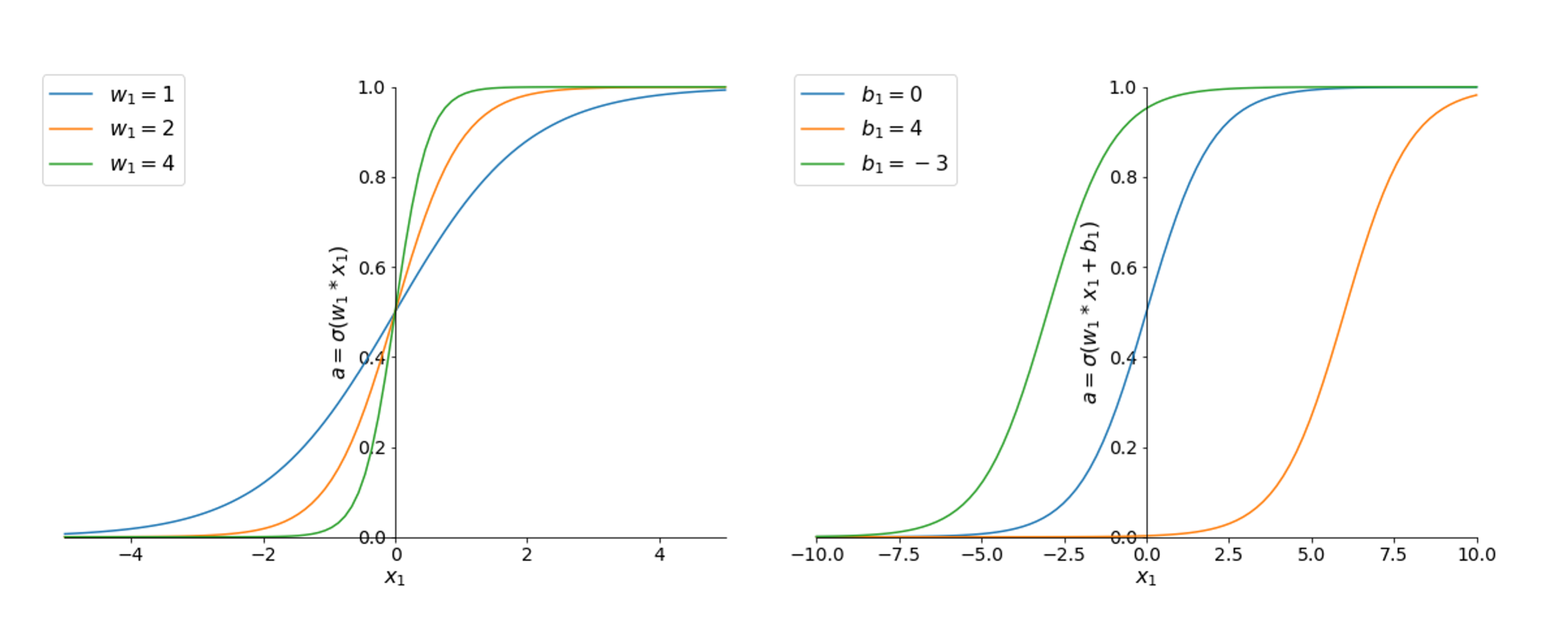

On the left of fig. 9 is the sigmoid function for 3 different values of the single weight w₁. You can see that if the NN changes the weight, this will simply change the steepness of the graph.
What about if when x₁ = 2, which gives a very strong activation for this neuron, we get a high cost function C(w). The network then decides that actually making this neuron’s activation close to 0 is good for C(w). From changing the weight alone it would never be able to make the activation of this neuron 0. This is where the bias term comes in.
From the right side of fig. 9 you can see that the bias term acts to shift the whole function along the x axis, but doesn’t change the overall shape of it. Therefore, you can now see that for an input of 2 you can get an activation close to 0 if b₁ > 0. Similarly, you can get the reverse situation if you’re bias term is negative.
Essentially, the bias term gives the NN more degrees of freedom with which to fit the data you have supplied it with.
What’s the need for a nonlinear activation function σ?
The short answer: without a nonlinear function, the multiplication of many weights and activations is simply a linear function of the input. Thus you can only solve problems that are linearly separable.
The long answer: what do we mean by linearly separable? This means that your problem can be solved using a hyperplane. A hyperplane in 2 dimensions is a.k.a a line, in 3 dimensions it is a.k.a a plane (like a piece of paper), and in general we call it a hyperplane.
For example, consider the left hand side of fig. 10 which contains two distinct groups coloured in green and orange. The blue line shows a possible hyperplane that solves this classification task. This is an example of a linearly separable problem


Now consider a problem which is not linearly separable. The easiest example of such a problem is the XOR gate. It has two inputs, let’s call them x₁ and x₂ and one output. The XOR problem is shown on the right-hand side of fig. 10. There is no hyperplane that perfectly separates out the two classes in this scenario.
How does this relate to the nonlinear function of the NN? Without the nonlinear function, the many layers of weight and activation multiplications could be represented by one big matrix M that maps the input vector, X to the output vector Y (i.e. M.X = Y). This matrix would be linear and thus would not be able to solve the XOR problem. Handwritten digit recognition is another such example of a non-linear problem. So, the nonlinear function breaks the linearity of NN so that they are able to solve more complex problems.


